
BASEMENT
Python 6주차 - 2 본문

파이썬 실습
1. 주식 가격 하락이 발생되기 전의 유지 시간(초) 계산
주식가격은 10이상 100이하
주식가격의 집합은 2이상 20이하
ex) 주식가격 : [59, 28, 84, 10, 74]
하락전 유지시간: [1, 2, 1, 1, 0]
import random

def stock_price(price):
    n = len(price)
    sec = [0] * n
    for i in range(n-1):
        for j in range(i+1,n):
            if price[i] > price[j]:
                break
        sec.append(j-i)
    return sec

if __name__ == "__main__":
    sp_n = int(input("enter number of stock price, 2-20>> "))
    sp = [random.randrange(10,100) for i in range(sp_n)]
    print()
    print(stock_price(sp))
2. 파일이름 정렬하기
파일은 HEAD, NUMBER, TAIL 세부분으로 구성됨
HEAD는 숫자가 아닌 문자로 이루어져 있으며 최소 한 글자 이상으로 구성
NUMBER는 한 글자에서 최대 다섯 글자 사이의 연속된 숫자로 구성, 앞쪽에 0이 올 수 있음
TAIL은 HEAD와 NUMBER를 제외한 나머지 부분, 숫자가 있을 수 도 있고 아무 글자 없을 수 도 있음
정렬기준
- HEAD 기준의 사전정렬을 먼저 하고 대소문자 구분 없음
- HEAD가 동일한 경우, NUMBER로 정렬. 4<0010<012<015<017 등, 4와 04는 동일값
- HEAD와 NUMBER가 동일하면 원래 입련된 순서로 정렬함
def file_sort(files):
    temp = dict()

    for file in files:
        hi,ni= 0,0
        for i in range(len(file)):
            if file[i].isnumberic():
                break
            else:
                hi = i
        for i in range(hi+1, len(file)):
            if file[i].isnumeric():
                ni = i
            else:
                break
        head, number = file[:hi+1].lower(), int(file[hi+1:ni+1])
        temp[file] = (head, number)

	result = [f_name for f_name, file_other in sorted(temp.items(), key=lambda x:(x[1][0], x[1][1]))]
	return result

if __name__ == "__main__":
    files = []
    while True:
        files.append(input("enter file name>> "))
        if files[-1] == '':
            file.pop()
            break

    print(file_sort(files))


# re 모듈 사용

import re

def file_sort(files):
    temp = [re.split(r"([0-9]+)", s) for s in files]
    print(temp)
    fs = sorted(temp, key=lambda x: (x[0].lower(), int(x[1])))
    print(fs)
    result = ["".join(s) for s in fs]
    return result
cf) sorted 함수의 key 사용법
key 없이 사용하는 경우 : 각 요소 순서대로 정렬
test = [(2,5,3), (10,3,8), (7,11,8), (1,7,100), (9,3,2)]

s_result = sorted(test)
print(s_result)

# 결과 : [(1, 7, 100), (2, 5, 3), (7, 11, 8), (9, 3, 2), (10, 3, 8)]
key 사용 시 : key 인자에 함수를 할당하고 해당 함수의 반환값을 비교하여 정렬함
test = [(2,5,3), (10,3,8), (7,11,8), (1,7,100), (9,3,2)]

s_result = sorted(test, key = lambda x: x[0])
ss_result = sorted(test, key = lambda x: x[1]) # 내림정렬은 -x[1]

print(s_result) # [(1, 7, 100), (2, 5, 3), (7, 11, 8), (9, 3, 2), (10, 3, 8)]
print(ss_result) # [(10, 3, 8), (9, 3, 2), (2, 5, 3), (1, 7, 100), (7, 11, 8)]
cf) 정규 표현식(regular expressions)
복잡한 문자열을 처리할 때 사용하는 기법
파이썬에서는 re 모듈 사용
정규표현식에 사용되는 메타 문자(meta characters) => . ^ $ * + { } ? [ ] | ( ) \
1) [ ]
[0-9] : 모든 숫자와 매치되는 의미
[^0-9] : 숫자가 아닌 것과 매치
[\t\n\r\f\v] : Whitespace 문자와 매치
[^\t\n\r\f\v] : Whitespace 문자가 아닌 것과 매치
[a-zA-Z0-9] : 문자 + 숫자와 매치
2) .
a.b : a와 b 사이에 줄바꿈 문자(\n)를 제외한 어떤 문자가 들어가도 모두 매치됨. a와 b 사이에 문자 하나 이상 필수
ex) aab, a0b는 매치, abc와는 매치x
3) *
go*gle
문자*문자 : 해당 메타문자 앞의 문자가 0번이상 무한대로 반복될 수 있음을 의미
ex) ggle, gogle, googel, goooooogle
4) +
go+gle : *와 같으나, 반복 회수가 최소 1번이상.
ex) gogle, google 매치, ggle 매치x
5) {}
{n,m}
n부터 m까지 반복 횟수지정
go{2}gle : google와 매치 o가 2번 반복
6) ?
go?gle : {0,1}을 의미, 0번~1번 반복
7) |
a|b : a또는 b와 매치되는 문자열 반환
8) ^
^ab : 처음 시작이 ab로 매치되는 문자열 반환
9) $
ab$ : 마지막이 ab로 매치되는 문자열 반환
cf) re 모듈
파이썬에서 정규표현식을 사용가능하게 해주는 내장 모듈
1) re 모듈 메서드
- match() : 문자열의 처음부터 정규식과 매치하는 지 확인. 일치하지 않는 경우 None, 매치되면 매치되는 객체 반환
- search() : 문자열 전체를 검사하여 정규식과 일치하는지 확인. 일치하지 않는 경우 None, 매치되면 매치되는 객체 반환. (match와 차이점 : 전체 문자열을 검사함)
- findall() : 정규식과 매치되는 모든 문자열을 리스트로 반환
- finditer() : 정규식과 매치되는 모든 문자열을 iterator 객체로 반환
# match / search 차이

import re

express = re.compile("[a-z]+")
print(express)
match_test1 = express.match("python")
print(match_test1)
print(match_test1.group())

match_test2 = express.search("4 times")		# 문자열의 처음이 숫자이므로 match를 사용하면 오류
print(match_test2)
print(match_test2.group())

match_test3 = express.match('version 3.0v')
print(match_test3)
print(match_test3.group())
# findall / finditer

import re

express = re.compile('[a-z]+')
findall_var1 = express.findall('python')
print(findall_var1)

findall_var2 = express.findall('5 times')
print(findall_var2)

findall_var3 = express.findall('python 3.8v')
print(findall_var3)

finditer_var1 = express.finditer('python version 3.8')
print(finditer_var1)
for i in finditer_var1:
    print(i)
    print(i.group())
2) compile 옵션
- DOTALL : \n 줄바꿈 문자 포함하여 매치
- IGNORECASE : 대소문자 구분없이 매치
- MULTILINE : 여러줄이 있을 때, 각 줄마다 문자열을 찾아서 매치
express = re.compile('a.b', re.DOTALL) # re.DOTALL : \n 포함
dotall_v = express.match('a\nb')
print(dotall_v.group())

dotall_v2 = re.match('c.f', 'c\nf', re.DOTALL)
print(dotall_v2)

express = re.compile('[a-z]+', re.IGNORECASE) # IGNORECASE : 대소문자 무시
ig_v1 = express.match("happy")
ig_v2 = express.match("Happy")
print(ig_v1, ig_v2)

ig_v3 = re.match('[a-z]+', 'Happy', re.IGNORECASE)
print(ig_v3)

express = re.compile('^Data\s\w+')
sentence = '''Data is important.
So, I study about data.
Data requires pre-processing.'''

print(express.findall(sentence))
print(re.findall('^Data\s\w+', sentence, re.MULTILINE))	# MULTILINE : 각 줄의 문자열을 확인
Numpy
배열
1) a[,] 와 a[:,:] 차이
import numpy as np

a = np.array([[1,2,3,4], [5,6,7,8], [9,10,11,12]])

row_r1 = a[1,:]
row_r2 = a[1:2,:]
print(row_r1, row_r1.shape)
print(row_r2, row_r2.shape)
print()

temp = a[1:,:3]
imsi = a[1:2,2]
print(imsi)
print(temp)

# 결과
[5 6 7 8] (4,)
[[5 6 7 8]] (1, 4)

[7]
[[ 5  6  7]
 [ 9 10 11]]
import numpy as np
a = np.array([[1,2,3,4], [5,6,7,8], [9,10,11,12]])
col_r1 = a[:,1]
col_r2 = a[:,1:2]
print(col_r1, col_r1.shape, col_r1.ndim)
print(col_r2, col_r2.shape, col_r2.ndim)
# 결과
[ 2 6 10] (3,) 1
[[ 2]
[ 6]
[10]] (3, 1) 2
2) Integer array indexing
import numpy as np

a = np.array([[1,2,3,4], [5,6,7,8], [9,10,11,12]])
print(a[[0,1,2], [0,1,0]])   # a[0,0], a[1,1], a[2,0]

b = np.array([a[0,0], a[1,1], a[2,0]])
print(b, b.shape)

print(a[[0,0], [1,1]])  # a[0,1], a[0,1]

# 결과
[1 6 9]
[1 6 9] (3,)
[2 2]
import numpy as np
a = np.array([[1,2,3], [4,5,6], [7,8,9], [10,11,12]])
print(a)
print()
b = np.array([0,2,0,1]) # a[0,0], a[1,2], a[2,0], a[3,1]
c = a[np.arange(4), b]
print(c, c.shape)
print()
a[np.arange(4), b] += 10
print(a)
# 결과
[[ 1 2 3]
[ 4 5 6]
[ 7 8 9]
[10 11 12]]
[ 1 6 7 11] (4,)
[[11 2 3]
[ 4 5 16]
[17 8 9]
[10 21 12]]
3) Boolean array indexing
import numpy as np

a = np.array([[1,2], [3,4], [5,6]])

bool_index = (a>2)
print(bool_index)

print(a[bool_index])
print(a[a>2])    # 조건이 True인 값만 리스트로 출력해줌

even_a = (a%2==0)
print(even_a)

print(a[even_a])
print(a[a%2==0])

# 결과
[[False False]
 [ True  True]
 [ True  True]]
[3 4 5 6]
[3 4 5 6]
[[False  True]
 [False  True]
 [False  True]]
[2 4 6]
[2 4 6]
4) dtype : Data type 확인
import numpy as np

a = np.array([3,4,5])
print(a.dtype)
b = np.array([3.0,4.0])
print(b.dtype)

c = np.array([1,2], dtype=np.float32)
print(c.dtype)
print(c)

# 결과
int32
float64
float32
[1. 2.]
실습
import numpy as np

a = np.array([[1,2,3,4], [5,6,7,8], [9,10,11,12]])
b = a[1:, ::2]
print(b, b.ndim, b.shape)
b[1,0] = 88   # 얕은 복사
print(a)

# 결과
[[ 5  7]
 [ 9 11]] 2 (2, 2)
[[ 1  2  3  4]
 [ 5  6  7  8]
 [88 10 11 12]]
import numpy as np
a = np.array([[1,2,3,4], [5,6,7,8], [9,10,11,12]])
b = a[::-1, ::-1]
print(b, b.ndim, b.shape)
# 결과
[[12 11 10 9]
[ 8 7 6 5]
[ 4 3 2 1]] 2 (3, 4)
5) reshape : 배열의 재구조화
import numpy as np

ary1 = np.arange(1,10)  # range와 같은 역할
print(ary1, ary1.ndim)
ary2 = ary1.reshape((3,3)) # 1차원 배열을 3 by 3 배열로 재구조화 함
print(ary2, ary2.ndim)

ary3 = np.array([[1,2,3,4], [5,6,7,8]])
re_ary3 = ary3.reshape((4,2))
print(re_ary3)

# 결과
[1 2 3 4 5 6 7 8 9] 1
[[1 2 3]
 [4 5 6]
 [7 8 9]] 2
[[1 2]
 [3 4]
 [5 6]
 [7 8]]
6) 배열의 연결 및 분할
- 연결 : concatenate, vstack, hstack
- 분할 : split, hsplit, vsplit
import numpy as np

ary1 = np.array([[1,2,3,4], [5,6,7,8]])
ary2 = np.array([[10,11,12,13], [14,15,16,17]])
ary3 = np.concatenate([ary1,ary2])  # 열의 수가 같아야 함. 세로 붙이기
ary4 = np.concatenate([ary1,ary2], axis=1) # 행의 수가 같아야함
print(ary3, ary3.shape)
print(ary4, ary4.shape)

# 결과
[[ 1  2  3  4]
 [ 5  6  7  8]
 [10 11 12 13]
 [14 15 16 17]] (4, 4)
[[ 1  2  3  4 10 11 12 13]
 [ 5  6  7  8 14 15 16 17]] (2, 8)
7) math
import numpy as np

a = np.array([[1,2], [3,4]])
b = np.array([[5,6], [7,8]])

print(a+b)
print(np.add(a,b))
print(a-b)
print(a*b)
print(a/b)
print(np.prod(a, axis=0))  # prod : 각 배열요소들의 곱. axis=0 열끼리 곱함, axis=1 행끼리 곱함
print(np.sqrt(a))          # sqrt : 루트

print(a.dot(b))
print(np.dot(a,b))        # dot : 내적
print(b.dot(a))
print(np.dot(b,a))

print(np.sum(a))
print(np.sum(a, axis=0))
print(np.sum(a, axis=1))

a_t = a.T                 # .T : 전치행렬
print(a_t)
8) 선형대수 함수
- linalg.det() : 행렬식
- linalg.inv() : 역행렬
- linalg.solve(a,b) : 연립방정식 해 구하기
import numpy as np

a = np.array([[1,2], [3,4]], dtype=np.float64)

a_det = np.linalg.det(a)  # 행렬식 계산
print(a_det)
a_inv = np.linalg.inv(a) # 역행렬 계산
print(a_inv)

# Ax = B의 방정식을 해결하는 메서드

a = np.array([[2,3], [4,1]])
b = np.array([[2], [5]])
x = np.linalg.solve(a,b)
print(x)
9) broadcasting
- 두 배열의 차원 수가 다르면 작은 차원을 가진 배열의 형상 앞쪽을 1로
- 두 배열의 형상이 모두 다르면 ,1을 가진 배열이 다른 배열과 동일
- 임의의 차원에서 크기가 일치하지 않고 1도 아니면 오류
import numpy as np

a = np.array([[1,2,3], [4,5,6], [7,8,9], [10,11,12]])
b = np.array([1,0,1])
c = np.empty_like(a)
print(c)
for i in range(4):
    c[i,:] = a[i,:] + b

print(c)

x = np.array([1,2,3])
w = np.array([4,5])
print(np.reshape(x,(3,1))*w)

# 결과
[[0 0 0]
 [0 0 0]
 [0 0 0]
 [0 0 0]]
[[ 2  2  4]
 [ 5  5  7]
 [ 8  8 10]
 [11 11 13]]
[[ 4  5]
 [ 8 10]
 [12 15]]
실습 - 2014년 시애틀의 강수량 데이터 활용
import numpy as np
import pandas as pd
import matplotlib.pyplot as plt

rainfall = pd.read_csv('Seattle2014.csv')['PRCP'].values   # PRCP 컬럼을 가져옴
inches = rainfall/25.4 # 25.4mm = 1 inches
plt.hist(inches, 40)
plt.show()
print("Number days without rain: ", np.sum(inches==0))
print("Number days with rain: ", np.sum(inches!=0))
print("Days with more than 0.5 inches: ", np.sum(inches>0.5))
print("Rainy days with < 0.1 inches: ", np.sum((inches>0) & (inches<0.2)))
10) numpy 수학함수
10-1) 연속 계산 메서드
- __add__(), add()
- 시그마 : cumsum
import numpy as np

temp = np.linspace(1,10,10) # default : 실수. dtype=np.int8로 정수 지정 가능
print(temp)
print(temp+temp)
print(temp.__add__(temp))
print(np.add(temp,temp))

# 결과
[ 1.  2.  3.  4.  5.  6.  7.  8.  9. 10.]
[ 2.  4.  6.  8. 10. 12. 14. 16. 18. 20.]
[ 2.  4.  6.  8. 10. 12. 14. 16. 18. 20.]
[ 2.  4.  6.  8. 10. 12. 14. 16. 18. 20.]
import numpy as np
temp = np.linspace(1,10,10)
sum_v = temp.sum()
cum_v = temp.cumsum()
print(sum_v);print(cum_v)
# 결과
55.0
[ 1. 3. 6. 10. 15. 21. 28. 36. 45. 55.]
10-2) 다차원 배열의 축에 따른 계산
- 열 기반으로 계산, 행 고정 : axis = 0
- 행 기반 계산, 열 고정 : axis = 1
import numpy as np

temp = np.arange(1,15).reshape(2,7)
print(temp)
print(np.sum(temp))
print(np.sum(temp, axis=0))
print(np.sum(temp, axis=1))

# 결과
[[ 1  2  3  4  5  6  7]
 [ 8  9 10 11 12 13 14]]
105
[ 9 11 13 15 17 19 21]
[28 77]
10-3) 파이
- prod, cumprod 메소드
import numpy as np

temp = np.linspace(1,10,10)
prod_v = temp.prod()
cump_v = temp.cumprod()
print(prod_v);print(cump_v)

# 결과
3628800.0
[1.0000e+00 2.0000e+00 6.0000e+00 2.4000e+01 1.2000e+02 7.2000e+02
 5.0400e+03 4.0320e+04 3.6288e+05 3.6288e+06]
10-4) 지수, 로그, 삼각함수
- 지수함수 : power, exp 함수 사용. exp는 밑이 자연상수 e인 경우
- cf) numpy의 power함수는 지수를 음수로 표시 불가능하여 ** 연산자를 이용하여 음수를 표시함
import numpy as np
import math
import matplotlib.pylot as plt

temp = np.arange(3,10, dtype=float)
print(np.power(10,2))
print(np.power(temp,2))
print(math.pow(temp[0],2))

print(math.pow(2,temp))   # 오류
print(np.power(2,temp))

# 밑이 e인 경우
print(np.exp(temp))
print(np.exp2(temp))  # 밑이 2인 경우만 해당
- 로그함수
- numpy의 log함수는 기본적으로 밑수가 e
- 상용로그는 log10 사용
- 밑수가 e 이외의 일반값인 경우 로그의 성질 이용
temp = np.arange(3,10)
print(np.log(temp))
print(math.log(temp[0]))

print(np.log10(temp))
print(np.log2(temp))
print(math.log(temp[0],2))

# 밑수가 일반값인 경우
base = 42
result = np.log(temp[0])/np.log(base)

exam = np.array([74088, 3111696])
result = np.log(exam)/np.log(base)
print(result)
- 삼각함수
- sin, cos, tan
- 각도를 라디안값으로 변환시켜주는 deg2rad 사용
np.sin(30)
np.sin(np.deg2rad(30))
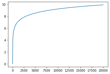
np.cos(np.deg2rad(np.arange(3,10)))# 지수, 로그 함수 그리기
import numpy as np
import matplotlib.pyplot as plt
x = np.linspace(1,10,300)
x_ = np.linspace(1,20000,300)
y = np.exp(x)
y_ = np.log(x_)
plt.plot(x,y)
plt.show()
plt.plot(x_,y_)
plt.show()
# 삼각 함수 그리기

x = np.linspace(-10,10,500)
y = np.sin(x)
plt.plot(x,y)
plt.show()
cf) subplots
여러 개의 그래프를 생성하고 싶은 경우
subplots(행,열) -> 두 개의 변수를 반환
하나는 전체 액자 figure에 대한 정보이며, 다른 하나는 액자 내 여러개에 대한 리스트 정보
각 액자에 그래프를 생성하려면 plt.plot()이 아닌 ax[i].plot()
fig, ax = plt.subplots(1,3)

plt.show()
subplots 속성을 활용하여 그래프 그리기
x = np.linspace(-10,10,500)
y = np.sin(x)

fig, ax = plt.subplots(figsize=(8,4))
ax.plot(x,y,linewidth=2,color='pink')
ax.spines['right'].set_color('none')
ax.spines['top'].set_color('none')
ax.spines['bottom'].set_position(('data',0))	# 좌표축을 0,0으로 이동
ax.spines['left'].set_position(('data',0))      # 좌표축을 0,0으로 이동
ax.set_xticks([-10,-5,5,10])	# x축 단위 바꾸기
ax.set_yticks([-1,-0.5,0.5,1])
ax.set_title('Sin Curve')
plt.show()
Pandas
Pandas 기본 정의
시계열 데이터 및 계측 인덱스 구조를 갖추고 있음
Numpy와 연동성이 높고, matplotlib를 기반으로 활용한 시각화 툴을 사용하여 데이터를 분석하는 툴
1) pandas 주 역할
- 데이터 입출력 기능 (csv, excel, RDB 등)
- 데이터 처리에 효율적 포맷 저장
- 데이터의 NaN(누락값) 처리
- 데이터의 일부 분리 또는 결합의 조작
- 데이터에 대한 통계 처리 및 회귀 처리 등
2) pandas의 데이터 타입
Numpy의 ndarray와 함께 쓰기 적합한 세가지 데이터 타입
- 1차원 : Series
- 2차원 : DataFrame
- 3차원 : Panel
3) Series
pd.Series(data, index=[index])
slicing은 리스트와 동일함
price = pd.Series([4000,3000,5000,2000])
print(price)
print(price.index)
print(price.values)

# 결과
0    4000
1    3000
2    5000
3    2000
dtype: int64
RangeIndex(start=0, stop=4, step=1)
[4000 3000 5000 2000]
import pandas as pd
fruit = pd.Series([4000,3000,5000,2000], index=['orange','mellon','kiwi','apple'])
print(fruit['mellon'])
print(fruit['mellon':'apple']) # index를 사용할 경우 apple까지 포함됨
print(fruit[1:3])
# 결과
3000
mellon 3000
kiwi 5000
apple 2000
dtype: int64
mellon 3000
kiwi 5000
dtype: int64# Series - 딕셔너리 형태
import pandas as pd
city_dict = {'Seoul':82, 'Pusan':90, 'Incheon':84, 'Gwangju':91}
city = pd.Series(city_dict)
print(city)
print(city.values)
print(city.index)
print(city['Pusan'])
# 결과
Seoul 82
Pusan 90
Incheon 84
Gwangju 91
dtype: int64
[82 90 84 91]
Index(['Seoul', 'Pusan', 'Incheon', 'Gwangju'], dtype='object')
90
4) DataFrame
딕셔너리를 데이터 프레임으로 사용하기 - 행, 열로 구성 (열을 리스트로 변환해줌)
city_dict = {'Seoul':[82], 'Pusan':[90], 'Incheon':[84], 'Gwangju':[91]}
city = pd.DataFrame(city_dict)
print(city)

# 결과
   Seoul  Pusan  Incheon  Gwangju
0     82     90       84       91
city_dict = {'Seoul':[82, '02'], 'Pusan':[90, '054'], 'Incheon':[84, '032'], 'Gwangju':[91, '043']}
city = pd.DataFrame(city_dict)
print(city)
# columns가 없는 경우 작성해줌
city = pd.DataFrame(city_dict, columns=['Seoul','Pusan','Incheon','Gwangju'])
print(city)
# 모든 도시의 지역코드, 0행 출력 시
print(city.iloc[0])
print(city.iloc[0].values)
# 결과
Seoul Pusan Incheon Gwangju
0 82 90 84 91
1 02 054 032 043
Seoul Pusan Incheon Gwangju
0 82 90 84 91
1 02 054 032 043
Seoul 82
Pusan 90
Incheon 84
Gwangju 91
[82 90 84 91]
4-1) DataFrame 객체 생성
code_dict = {'Seoul':82, 'Pusan':90, 'Incheon':84, 'Gwangju':91}
population_dict = {'Seoul':9845336, 'Pusan':3465407, 'Incheon':2951629, 'Gwangju':1463100}
code = pd.Series(code_dict)
population = pd.Series(population_dict)
city = pd.DataFrame({'code':code, 'population':population})
print(city)
print(city.index)
print(city.values)
print(city.columns)
print(city['code'])

# 결과

         code  population
Seoul      82     9845336
Pusan      90     3465407
Incheon    84     2951629
Gwangju    91     1463100
Index(['Seoul', 'Pusan', 'Incheon', 'Gwangju'], dtype='object')
[[     82 9845336]
 [     90 3465407]
 [     84 2951629]
 [     91 1463100]]
Index(['code', 'population'], dtype='object')
Seoul      82
Pusan      90
Incheon    84
Gwangju    91
Name: code, dtype: int64
import random
df = pd.DataFrame(np.random.randn(6,4), index=[1,2,3,4,5,6], columns=['A','B','C','D'])
print(df.head(3))
print(df.index)
print(df.columns)
print(df.values)
print(df.describe()) # 각 열의 통계적 계요
print(df.sort_values(by='B', ascending=False)) # B열을 기준으로 정렬
print(df.loc[2,['A','B']]) # 특정 index와 열에 해당되는 데이터 내용 확인
print(df[df.A>0]) # 컬럼 A에서 0보다 큰 행의 값 확인. df.A 대신 df['A']로 표기 가능
df2 = df.copy() # 깊은복사
df2['E'] = ['one', 'two', 'three', 'four', 'five', 'six'] # 새로운 컬럼 E 추가
print(df2)
# 결과
A B C D
1 0.454240 0.576628 2.178587 -0.021071
2 -0.982265 -0.872982 -0.377664 0.241053
3 -0.433437 2.145139 -0.381985 0.190848
Int64Index([1, 2, 3, 4, 5, 6], dtype='int64')
Index(['A', 'B', 'C', 'D'], dtype='object')
[[ 0.45424004 0.57662778 2.17858681 -0.02107089]
[-0.98226491 -0.8729823 -0.37766399 0.24105266]
[-0.43343732 2.14513865 -0.38198471 0.19084789]
[ 0.14338704 0.30708815 -0.60083904 -0.30223057]
[ 0.22294121 -0.32771942 -0.17002379 -0.65413048]
[ 1.18633211 1.55245175 0.35941724 0.63016333]]
A B C D
count 6.000000 6.000000 6.000000 6.000000
mean 0.098533 0.563434 0.167915 0.014105
std 0.745445 1.131661 1.037758 0.449470
min -0.982265 -0.872982 -0.600839 -0.654130
25% -0.289231 -0.169018 -0.380905 -0.231941
50% 0.183164 0.441858 -0.273844 0.084889
75% 0.396415 1.308496 0.227057 0.228501
max 1.186332 2.145139 2.178587 0.630163
A B C D
3 -0.433437 2.145139 -0.381985 0.190848
6 1.186332 1.552452 0.359417 0.630163
1 0.454240 0.576628 2.178587 -0.021071
4 0.143387 0.307088 -0.600839 -0.302231
5 0.222941 -0.327719 -0.170024 -0.654130
2 -0.982265 -0.872982 -0.377664 0.241053
A -0.982265
B -0.872982
Name: 2, dtype: float64
A B C D
1 0.454240 0.576628 2.178587 -0.021071
4 0.143387 0.307088 -0.600839 -0.302231
5 0.222941 -0.327719 -0.170024 -0.654130
6 1.186332 1.552452 0.359417 0.630163
A B C D E
1 0.454240 0.576628 2.178587 -0.021071 one
2 -0.982265 -0.872982 -0.377664 0.241053 two
3 -0.433437 2.145139 -0.381985 0.190848 three
4 0.143387 0.307088 -0.600839 -0.302231 four
5 0.222941 -0.327719 -0.170024 -0.654130 five
6 1.186332 1.552452 0.359417 0.630163 six
5) 누락데이터 표현
import numpy as np
import pandas as pd
np.nan 또는 None
ex) df = pd.Series([1,2,np.nan,4,5,None])
5-1) 누락데이터 처리
- 누락데이터 삭제
dropna(<axis='columns' or 'rows'>, <how='all' or 'any'>, <thresh=누락이 아닌 갯수>)
ex) df.dropna() / df.dropna(axis='cloumns') / df.dropna(axis='columns', how='all')
- 누락데이터를 다른 데이터값으로 대체
fillna(data, <method='ffill' or 'bfill'>, <axis='columns' or 'rows'>)
ex) df.fillna(0) / df.fillna(method='ffill') / df.fillna(method='bfill', axis=1)
data = pd.Series(['a','b','c',None,'e'], index=[1,3,5,7,9])
print(data.dropna())
data = pd.DataFrame([[1,np.nan,3,4], [5,6,None,8], [np.nan,10,11,12]], index=['a','b','c'], columns=['first','second','third','forth'])
print(data)
print(data.fillna(0))
print(data.fillna(method='ffill', axis=1))

# 결과
1    a
3    b
5    c
9    e
dtype: object
   first  second  third  forth
a    1.0     NaN    3.0      4
b    5.0     6.0    NaN      8
c    NaN    10.0   11.0     12
   first  second  third  forth
a    1.0     0.0    3.0      4
b    5.0     6.0    0.0      8
c    0.0    10.0   11.0     12
   first  second  third  forth
a    1.0     1.0    3.0    4.0
b    5.0     6.0    6.0    8.0
c    NaN    10.0   11.0   12.0
6) groupby
같은 값을 하나로 묶어 통계 또는 집계결과를 얻기 위해 사용함
df = pd.DataFrame({
	'city':['부산','부산','부산','부산','서울','서울,'서울'],
    'fruits':['apple','orange','banana','banana','apple','apple','banana'],
    'price':[100,200,250,300,150,200,400],
    'quantity':[1,2,3,4,5,6,7]
})

df.groupby('city').mean()
df.groupby(['city', 'fruits']).mean()
1) get_group() : 그룹 안에 데이터를 확인하고 싶은 경우
df.groupby('city').get_group('부산')2) size() : 각 그룹의 사이즈 확인
df.groupby('city').size()
df.groupby('city').size()['부산']
3) agg() : Aggregation으로 groupby.mean()과 유사
df.groupby('city').agg(np.mean)cf) 가격 평균과 수량의 합계를 동시에 구하는 경우, agg사용
def my_mean(s):
	return np.mean(s)
df.groupby('city').agg({'price':my_mean, 'quantity':np.sum})
'Programming > Python' 카테고리의 다른 글
| Python 7주차 - 2 (0) | 2020.08.03 |
|---|---|
| Python 7주차 - 1 (0) | 2020.07.29 |
| Python 6주차 - 1 (0) | 2020.07.26 |
| Python 5주차 (0) | 2020.07.26 |
| Python 4주차 - 2 (0) | 2020.07.12 |


